How to use computer vision to crop images
The problem of cropping
Cropping of images is often one of the last things to do before publishing an article. We have to finalise all images and text content before knowing how much space to use for each component and how it all fits together.
In digital publishing, the same images are often reused in a multitude of shapes and sizes for different channels. A typical blog post or news article will have a main article view. But in a responsive page layout, the images often will have different shapes on different screen sizes. With a website redesign, legacy content might also have to be converted to a new layout in bulk. That could involve a new shape for primary and supporting images. There’s section front pages, search result pages, «related content»-teasers and social media previews. Many of these layouts require that images must be cropped into a specific shape.
Even a human designer or editor is doing the image cropping manually, it can be difficult to know which parts of a photo to crop away and which parts to keep.
An Algorithm of Aesthetics
When there’s a large set of images that must be cropped, it’s sometimes unfeasible to manually decide how to best crop each individual photo. Instead we can use an automated process to classify images and determine which features and point of interest that is most important, and as a consequence, which sections of the image that are less interesting.
In this article I’ll show how we can use the open source OpenCV computer vision library and the Python programming language to analyze photos to automate image cropping.
The Open Source Computer Vision library
OpenCV is a very large library of tools and algoritms for computer vision. It’s written in C++ and has bindings for Java, C++ and Python. Like many other scientific packagages that are written by and for academics and scientist, the documentation and the apis can be somewhat hard to understand without the relevant academic background.
Installing OpenCV is also much less straightforward than your typical python package. To use the latest version with python 3 support you have to install a lot of supporting libraries and configure and build OpenCV itself using cmake. There are also prebuilt versions available for some versions and operating systems. I found the installation guides at pyimagesearch.com very helpful when to get opencv3.0 and python3.5 bindings installed on ubuntu.
The OpenCV library gives you a very large toolbox of algorithms for doing all sorts of computer vision, video and image analysis. In this article I’m just going to use two of them: The ORB keypoint detector and descriptor extractor and the Viola-Jones object detection framework (Haar Cascade Classifier).
When reading the OpenCV documentation, you’ll run into a lot of academic terms like «Haar Cascade» and acronyms such as BRIEF (Binary Robust Independent Elementary Features). All of these are described in various scientific papers, and to really undestand how the algorithms work takes a lot of effort. The good news is that you don’t really have to understand how everything works to be able to actually use OpenCV. A good place to find beginner friendly tutorials is pyimagesearch.com.
Playing around with OpenCV in Jupyter
Since OpenCV is a computer vision library, you can play around with images and
algorithms and get quick visual results. Algorithms such as Viola-Jones and ORB are optimized for speed so that they can be used for real time video. Thus they are can also process static images very fast.
Whenever I want to learn a new python library, I use Jupyter notebooks to do some exploratory programming. This is also a tool that is used a lot in academia and science, since it’s very well suited for exploring data and sharing code.
Jupyter can also be used to edit markdown. In fact this blog post is written in jupyter (you can see the source here).
The apis and output data structures in OpenCV do not seem to follow any common
structure, so for a python programmer it can be quite confusing to use. Since I
want to use both Viola-Jones (cv2.CascadeClassifier) and ORB
(cv2.ORBClassifier) to detect salient features or points of interest in images.
Feature detector interface
Since the OpenCV apis are complex and each algorithm is implemented differently, we’ll create some wrapper classes that presents a uniform interface. This would be an example of the Facade or Adapter design pattern.
We’ll start by defining a base class that defines the interface that all the detectors will use. To make it more explicit we’ll define it as an Abstract Base Class, using the standard library abc module. I’m also using type annotations, which is a fairly new feature in python 3.
import abc   # abstract base classes
from typing import List  # type annotations
from utils.cropengine import Feature  # I'll explain this one soon.

FileName = str  # type alias

class FeatureDetector(abc.ABC):
	"""Abstract base class for the feature detectors."""

	@abc.abstractmethod
	def __init__(self, n:int, size:int) -> None:
		...

	@abc.abstractmethod
	def detect_features(self, fn: FileName) -> List[Feature]:
		"""Find the most salient features of the image."""
		...
All our feature detector classes will be subclasses of FeatureDetector and must override the detect_features method, using the same method signature.
Here’s the function we’ll use to prepare image files for image analyzis. The function reads an image file and optionally resamples it to a standard image size. This is useful for normalizing images to a standard size, as well as for performance.
import cv2	# The opencv python bindings
import numpy  # Python scienticic computing library

# OpenCv represents all images as n-dimensional numpy arrays.
# For clarity and convenience, we'll just call it "CvImage"
CVImage = numpy.ndarray

def opencv_image(fn: str, resize: int=0) -> CVImage:
	"""Read image file to grayscale openCV int array.

	The OpenCV algorithms works on a two dimensional
	numpy array integers where 0 is black and 255 is
	white. Color images will be converted to grayscale.
	"""
	cv_image = cv2.imread(fn)
	cv_image = cv2.cvtColor(
		cv_image, cv2.COLOR_BGR2GRAY)
	if resize > 0:
		w, h = cv_image.shape[1::-1]  # type: int, int
		multiplier = (resize ** 2 / (w * h)) ** 0.5
		dimensions = tuple(
			int(round(d * multiplier)) for d in (w, h))
		cv_image = cv2.resize(
			cv_image, dimensions,
			interpolation=cv2.INTER_AREA)
	return cv_image

def resize_feature(feature: Feature, cv_image: CVImage) -> Feature:
	"""Convert a Feature to a relative coordinate system.

	The output will be in a normalized coordinate system
	where the image width and height are both 1.
	Any part of the Feature that overflows the image
	frame will be truncated.
	"""
	img_h, img_w = cv_image.shape[:2]  # type: int, int
	feature = Feature(
		label=feature.label,
		weight=feature.weight / (img_w * img_h),
		left=max(0, feature.left / img_w),
		top=max(0, feature.top / img_h),
		right=min(1, feature.right / img_w),
		bottom=min(1, feature.bottom / img_h),
	)
	return feature
Let’s try this function on an example image. First we use a utility function show_image to display the source image. Then, we’ll convert it to a very low resolution numpy array, and then we’ll convert the array back to an image format, so we can compare with the original.
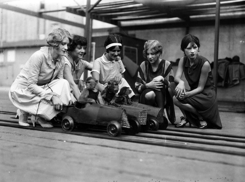
monkey_race = './monkey-race-wide.jpg'
show_image(monkey_race)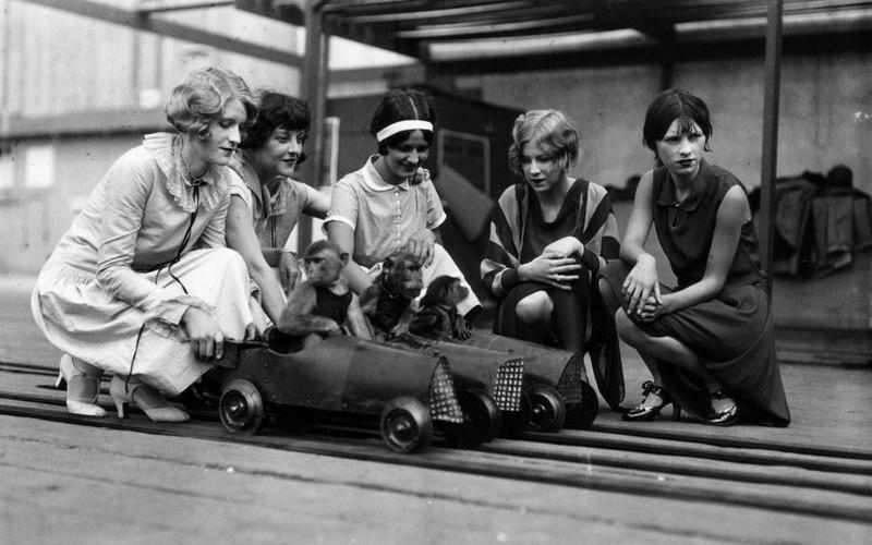
img_array = opencv_image(monkey_race, 6)
show_image(img_array) # convert to png and display
Let’s see what the raw numpy array looks like.
img_array # This is the data type that opencv uses.array([[208, 181, 137, 85, 68, 58, 52, 68],
[179, 149, 96, 116, 55, 98, 83, 79],
[196, 170, 142, 97, 63, 76, 54, 46],
[129, 109, 41, 55, 53, 50, 36, 86],
[155, 155, 157, 139, 133, 127, 114, 110]], dtype=uint8)When we prepare the image for a computer vision algorithm, we’ll try to find the smallest input size that still gives us acceptable results. Shrinking the input image can save a lot of execution time, but at some point, downsampling will result in low quality output from the algorithms. In this case, there’s not much useful data left from the original image.
Output data
We know what the input looks like, let’s figure out what output data we expect from our feature detector. To make the output portable, we’ll ultimately store and transmit it in json format. It will be an array of objects.
# This is what the json data looks like.
# Conveniently it's also valid python code.
data = [
  {
	"label": "keypoint one",
	"x": 0.25,
	"y": 0.25,
	"width": 0.30,
	"height": 0.50,
	"weight": 2
  },
  {
	"label": "keypoint two",
	"x": 0.20,
	"y": 0.20,
	"width": 0.15,
	"height": 0.25,
	"weight": 1
  }
]
Each feature is represented as a rectangle in a coordinate system where (0, 0) is the upper left corner of the image and (1, 1) is the lower right corner of the image. This is convenient since we are going to use this data to render html and svg graphics.
labelis a string that will be used as a css class for the feature, so we can distinguish various types of features.xandyare the coordinates of the upper left corner of the featureweightis a quantity representing the relative importance or saliency of a given feature.
To visualize these feature, we’ll use reactjs and node to create a svg and html widget.
# Renders the widget with react, redux and node.js
features = [Feature.deserialize(item) for item in data]
show_features(monkey_race, features)As you can see, the Feature class can be serialized and deserialized, which makes it possible to convert to json and back. In addition, the class implements implements some dunderscore methods, such as __add__, __mul__ and __and__ so that we can perform operations using the built-in operators +, *, & etc.
Multiplication will change the size and weight of the Feature, but the center point and label will not change.
features[0] * 0.4Feature(weight=0.8, label='keypoint one', left=0.34, top=0.4, right=0.46, bottom=0.6)
Adding two features together will give us a new Box that circumscribes both features.
features[0] + features[1]Box(left=0.2, top=0.2, right=0.55, bottom=0.75)
The & operator will return a Box that is the intersection of the two operand features.
features[0] & features[1]Box(left=0.25, top=0.25, right=0.35, bottom=0.45)
Putting it together
For convenience we’ll add two useful static methods to the FeatureDetector class
FeatureDetector._opencv_image = staticmethod(opencv_image)
FeatureDetector._resize_feature = staticmethod(resize_feature)
Let’s make an actual feature detector class. We’ll not use any computer vision algoritms. Instead we’ll just return some mock features. The widget sort of resembles a gun sight, so why not let it look even more so.
class MockFeatureDetector(FeatureDetector):

	"""Example feature detector interface."""

	def __init__(self, n: int=3, size: int=200) -> None:
		self._number = n
		self._size = size
		self._circles = [m / n for m in range(1, n + 1)]

	def detect_features(self, fn: FileName) -> List[Feature]:
		"""Concentric features at center of the image"""
		cv_image = self._opencv_image(fn, self._size)
		img_h, img_w = cv_image.shape[:2]
		middle = Feature(0, 'mock keypoint', 0, 0, img_w, img_h)
		middle.width = middle.height = min(img_w, img_h)
		middle = self._resize_feature(middle, cv_image)
		return [middle * size for size in self._circles]

def show_features(image_file: FileName, detector: FeatureDetector):
	features = detector.detect_features(image_file)
	return render(image_file, features)

dessau_image = './Henri-Cartier-Bresson-Dessau-1945.jpg'
detect_and_show(dessau_image, MockFeatureDetector())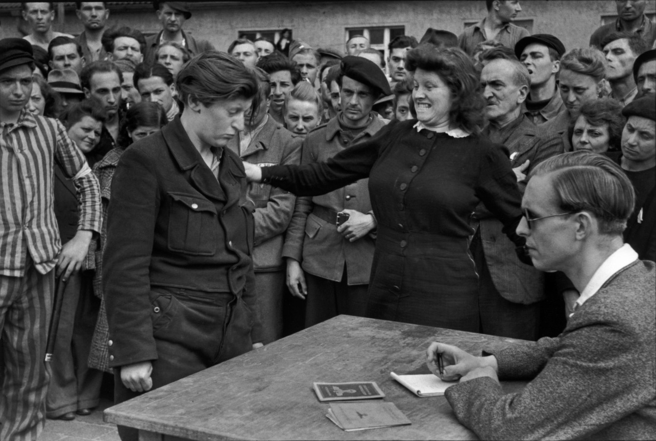
Excellent. But still quite useless. Let’s try to use an actual computer vision algorithm to find some real features.
We want to emulate human vision. The goal is to guess what elements in a photo would look most interesting to a human.
For a typical photo, we can take advantage of the fact that the photographer is a human. He or she has looked at a scene and tried to capture something of interest in the photo. That means that the most important motive is usually in focus and clearly visible. Photographers also try to avoid visual clutter in their photos by keeping distracting elements out of focus or out of the image altogether.
Therefore, any element that has strong contrast and sharp edges is usually a deliberate choice from the photographer. It’s somthing interesting.
In computer vision terms, we are looking for what’s called «corners», «points of interest» or «keypoints». There are many algorithms that we can use to detect and describe keypoints. Finding keypoints is used as an initial step in many computer vision applications, for instance tracking moving objects in a video stream, or finding similarities between two images.
For our use, we only want to find a small number of eye catching keypoints in our image. For this we’ll use an algorithm called ORB.
ORB is short for «Oriented FAST and Rotated BRIEF». It’s one of several feature detection implementations that are included with opencv. It’s main advantages for our purpose is that it’s very fast, and that it return values give us both coordinates, size and strength of the keypoints that it detects.
Here’s a simple usage of opencv’s orb detector. We’ll find five keypoints in an image.
image_array = cv2.imread(dessau_image)
orb_detector = cv2.ORB_create(3)
keypoints = orb_detector.detect(image_array)
keypoints
[<KeyPoint 0x7fc993aa0ba0>, <KeyPoint 0x7fc993aa0b10>, <KeyPoint 0x7fc993aa0ab0>]
Let’s inspect the Keypoint object to see what it contains.
kp = keypoints[0]
print('\n'.join('kp.{:10}: {}'.format(attr, getattr(kp, attr))
				for attr in dir(kp) if not attr.startswith('_')))
kp.angle : 277.11895751953125 kp.class_id : -1 kp.convert : <built-in method convert of type object at 0x7fc9c09ca180> kp.octave : 0 kp.overlap : <built-in method overlap of type object at 0x7fc9c09ca180> kp.pt : (853.0, 267.0) kp.response : 0.0019969299901276827 kp.size : 31.0
OpenCVs python bindings unfortunately doesn’t provide any docstrings, but the online documentation explains what the values mean.
The ones we care about are KeyPoint.pt, KeyPoint.response and KeyPoint.size.
Data structure for salient point detectors.
ptcoordinates of the keypoint
sizediameter of the meaningful keypoint neighborhood
responsethe response by which the most strong keypoints have been selected. Can be used for further sorting or subsampling
The docs also explains the initialization parameters for the ORB detector.
Class implementing the ORB (oriented BRIEF) keypoint detector and descriptor extractor.
The algorithm uses FAST in pyramids to detect stable keypoints, selects the strongest features using FAST or Harris response, finds their orientation using first-order moments and computes the descriptors using BRIEF (where the coordinates of random point pairs (or k-tuples) are rotated according to the measured orientation).The maximum number of features to retain.
nfeaturesThe maximum number of features to retain.
scaleFactorPyramid decimation ratio, greater than 1. scaleFactor==2 means the classical pyramid, where each next level has 4x less pixels than the previous, but such a big scale factor will degrade feature matching scores dramatically. On the other hand, too close to 1 scale factor will mean that to cover certain scale range you will need more pyramid levels and so the speed will suffer.
patchSizesize of the patch used by the oriented BRIEF descriptor. Of course, on smaller pyramid layers the perceived image area covered by a feature will be larger
This documentation is actually quite straightforward. But to dig deeper into how the algorithm works, we either have to read the C++ source code or the academic journals and math formulae behind the algorithms.
Another way to figure it out is to just use the bindings and see what results we can get.
Keypoint detector implementation
This is my python wrapper class for the ORB detector.
I’ve experimented and tweaked the default parameters in the __init__ method until it found features that are fairly similar to what a human being might find salient.
class KeypointDetector(FeatureDetector):

	"""Feature detector using OpenCVs ORB algorithm"""

	LABEL = 'ORB keypoint'

	def __init__(self, n: int=10, padding: float=1.0,
				 imagesize: int=200, **kwargs) -> None:
		self._imagesize = imagesize
		self._padding = padding
		kwargs = {
			"nfeatures": n + 1,
			"scaleFactor": 1.5,
			"patchSize": self._imagesize // 10,
			"edgeThreshold": self._imagesize // 10,
			"scoreType": cv2.ORB_FAST_SCORE,
			**kwargs,
		}
		self._detector = cv2.ORB_create(**kwargs)

	def detect_features(self, fn: str) -> List[Feature]:
		"""Find interesting keypoints in the image."""
		cv_image = self._opencv_image(fn, self._imagesize)
		keypoints = self._detector.detect(cv_image)
		features = []
		for kp in keypoints:
			ft = self._kp_to_feature(kp)
			ft = self._resize_feature(ft, cv_image)
			features.append(ft)
		return sorted(features, reverse=True)

	def _kp_to_feature(self, kp: cv2.KeyPoint) -> Feature:
		"""Convert KeyPoint to Feature."""
		x, y = kp.pt
		radius = kp.size / 2
		weight = radius * kp.response ** 2
		return Feature(
			label=self.LABEL,
			weight=weight,
			left=x - radius,
			top=y - radius,
			right=x + radius,
			bottom=y + radius
		) * self._padding
Before going through this code, let’s look at the output it produces.
bike_image = './Henri-Cartier-Bresson-Hyeres-France-1932.jpg'
detector = KeypointDetector()
detect_and_show(bike_image, detector)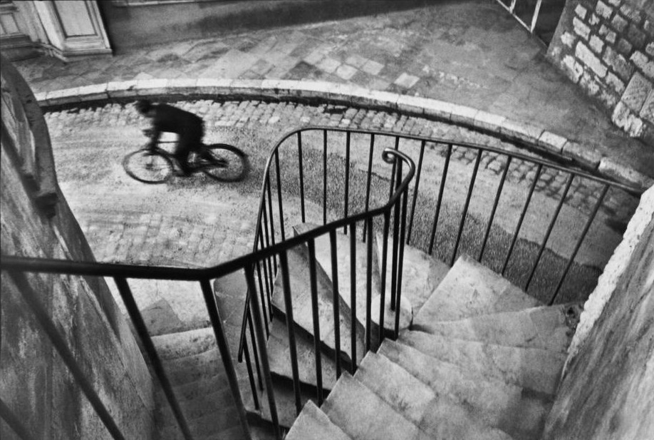
What’s worth noticing is that the keypoints that we have detected are areas of the image that have a sharp contrast between darkness and brightness. The main motive in the potography is the bicyclist. Even thought there’s significant motion blur, the keypoint with the highest relevance is on the bicyclist.
This is because we have downsampled the image to aproximately 400 pixels, which has an effect similar to looking at the scene from far away. Only the large details are preserved.
This is what the downsampled image looks like:
show_image(opencv_image(bike_image, 200))If we try this without downsampling the image, the strongest keypoints is on the railing, because that’s the part of the photo where we find the highest contrast and sharpness. But it’s not really what a human would find most interesting.
detector2 = KeypointDetector(imagesize=2000)
detect_and_show(bike_image, detector2)If we increase the number of keypoints and reduces their size, we get an better impression of the kind of keypoint that ORB is designed to find.
detector3 = KeypointDetector(
	n=100, imagesize=2000, patchSize=30, edgeThreshold=30)
detect_and_show(bike_image, detector3)For most photos, this image detector gives quite good results. But unlike a human it doesn’t really see what’s in the photo. In the photo below, the strongest feature is someone’s hand.
detect_and_show(dessau_image, detector)The next step is to try to analyze the actual contents of the image and detect human faces with using the Viola-Jones algorithm.
This problem is quite different from the last one. In order for an algorithm to detect faces in an image, it has to learn what a face looks like first.
The Viola-Jones algorithm uses a cascading of simple rules called «Haar like features». The cascade is produced by a learning algorithm from a large set of training images. The learning algorithm can also be trained to recognize other objects, as long as the objects always are depicted from the same angle and orientation.
OpenCV comes with several pre-trained Haar cascade files that can be used to recognize human faces, eyes, bodies etc. That’s very useful, because training a classifier takes a lot of time, processing power and requires a library of training images.
Running a simple detection is straightforward.
# Prepare the image and initilize the classifier
# In this case we're looking for noses.
image_array = cv2.imread(monkey_race)
cascade_file = '/usr/local/share/OpenCV/haarcascades/haarcascade_frontalcatface.xml'
viola_jones_classifier = cv2.CascadeClassifier(cascade_file)

# Detect noses!
viola_jones_classifier.detectMultiScale(image_array)
array([[602, 105, 49, 49]], dtype=int32)
Each row in the result array is a match. The numbers are [left, top, width, height] of a bounding rectangle. A classifier always produces matches with a specific shape, but like with the ORB algorithm, the algorithm returns matches in multiple sizes.
Viola-Jones can be fast enough to find faces in real time video streams. But does not always correctly identify faces, and can also produce false positives. By tweaking the parameters we can find a good balance between speed and accuracy.
Running it on typicial portrait photos, we can easily get very good results. False negatives can happen because the faces in our photo look different from the ones in the training data. Variations in rotation, facial hair, light conditions and ethnicity and skin colour might result in false negatives.
Most images will also result in several false positives. The algorithm will often recognize a face in some quite unexpected places. To eliminate most of these false negatives, the final classification is based on several passes over the image. Each pass is done with a different size detection window.
Face detector and Cascade classifier
The Detector class in this case is more complicated than the ORB detector. To find both frontal faces and profile faces, this feature detector uses combines several cascade classifiers. We’ll start by defining a helper class to wrap the cv2 CascadeClassifier.
class Cascade:

	"""Wrapper for Haar cascade classifier"""

	_DIR = '/usr/local/share/OpenCV/haarcascades/'

	def __init__(self, label: str, fn: FileName,
				 size: float=1, weight: float=100) -> None:
		self.label = label
		self.size = size
		self.weight = weight
		self._file = self._DIR + fn
		self.classifier = cv2.CascadeClassifier(self._file)
		if self.classifier.empty():
			msg = ('The input file: "{}" is not a valid '
				   'cascade classifier').format(self._file)
			raise RuntimeError(msg)
class FaceDetector(FeatureDetector):
"""Face detector using OpenCVs Viola-Jones algorithm and
and Haar cascade training data files classifying human
frontal and profile faces."""
_CASCADES = [
Cascade('frontal face',
'haarcascade_frontalface_default.xml',
size=1.0, weight=100),
Cascade('alt face',
'haarcascade_frontalface_alt_tree.xml',
size=0.8, weight=100),
Cascade('profile face',
'haarcascade_profileface.xml',
size=0.9, weight=50),
]
def __init__(self, n: int=100, padding: float=1.2,
imagesize: int=610, **kwargs) -> None:
self._number = n
self._imagesize = imagesize
self._padding = padding
self._cascades = self._CASCADES
minsize = max(25, imagesize // 25)
self._kwargs = {
"minSize": (minsize, minsize),
"scaleFactor": 1.1,
"minNeighbors": 5,
}
self._kwargs.update(kwargs)
def detect_features(self, fn: FileName) -> List[Feature]:
"""Find faces in the image."""
features = [] # type: List[Feature]
cv_image = self._opencv_image(fn, self._imagesize)
for cascade in self._cascades:
padding = self._padding * cascade.size
detect = cascade.classifier.detectMultiScale
faces = detect(cv_image, **self._kwargs)
for left, top, width, height in faces:
weight = height * width * cascade.weight
face = Feature(
label=cascade.label,
weight=weight,
left=left,
top=top,
right=left + width,
bottom=top + height,
)
face = face * padding
face = self._resize_feature(face, cv_image)
features.append(face)
return sorted(features, reverse=True)[:self._number]Face detection output
To make it easier to see which cascade classifier resulted in which match, I use different sizes and symbols for each Classifier. As we can see there are no false positives, but the photo also contains several faces that were not detected.
detect_and_show(dessau_image, FaceDetector())The most significant parameters we pass to detectMultiscale are these:
CascadeClassifier.detectMultiscale()
scaleFactorParameter specifying how much the image size is reduced at each image scale.
minNeighborsParameter specifying how many neighbors each candidate rectangle should have to retain it.
If we remove the minNeighbors constraint, we can see the overlapping matches that would be condensed into a single match by the algorithm, and also a lot of stray false positives.
generous_face_detector = FaceDetector(minNeighbors=0)
detect_and_show(dessau_image, generous_face_detector)The generous detector only produces a few more true positives for each extra false negative. It will detect «faces» in almost any photo.
detect_and_show(bike_image, generous_face_detector)In comparison, the default FaceDetector produces very good results if the faces in the input image are clearly visible and not rotated.
detect_and_show('Henri-Cartier-Bresson-Alicante-1932.jpg', FaceDetector())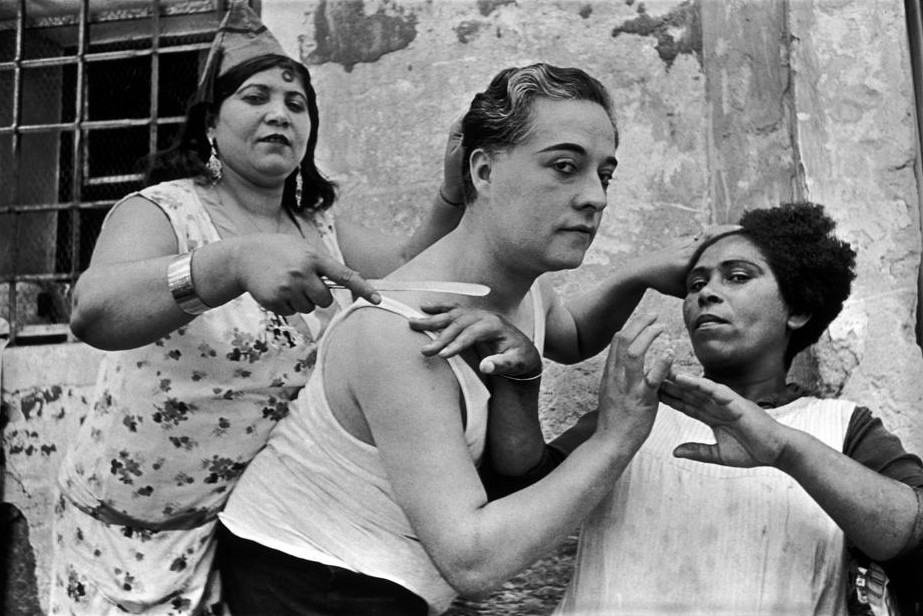
We can also make a face detector instance to detect just a single face, which will be the largest match found.
detect_and_show('Henri-Cartier-Bresson-Alicante-1932.jpg', FaceDetector(1))The face detector is good for images where the faces are the center of attention, but it’s completely useless on images where there’s no faces. To create a general purpose feature detector, we can combine both algorithms into a hybrid strategy feature detector.
Combined feature detector
This detector combines the power of both algorithms. We don’t need to write much code to do so, since we can reuse the FaceDetector and KeypointDetector through composition.
class HybridDetector(FeatureDetector):

	"""Detector using a hybrid strategy to find salient
	features in images.

	Tries to detect_features faces first. If the faces are
	small relative to the image, will detect_features
	keypoints as well. If no faces are detected, will fall
	back to a pure KeypointDetector."""

	BREAKPOINT = 0.15

	def __init__(self, n=10) -> None:
		self.primary = FaceDetector(n, padding=1.5)
		self.fallback = KeypointDetector(n, padding=1.2)
		self.breakpoint = self.BREAKPOINT
		self._number = n

	def detect_features(self, fn: FileName) -> List[Feature]:
		"""Find faces and/or keypoints in the image."""
		faces = self.primary.detect_features(fn)
		if faces and sum(faces).size > self.breakpoint:
			return faces
		features = faces + self.fallback.detect_features(fn)
		return features[:self._number]
This detector is ideal for images just one or a few faces which only covers a small part of the image.
detect_and_show('./Gordon-Parks-New-York-1958.jpg', HybridDetector())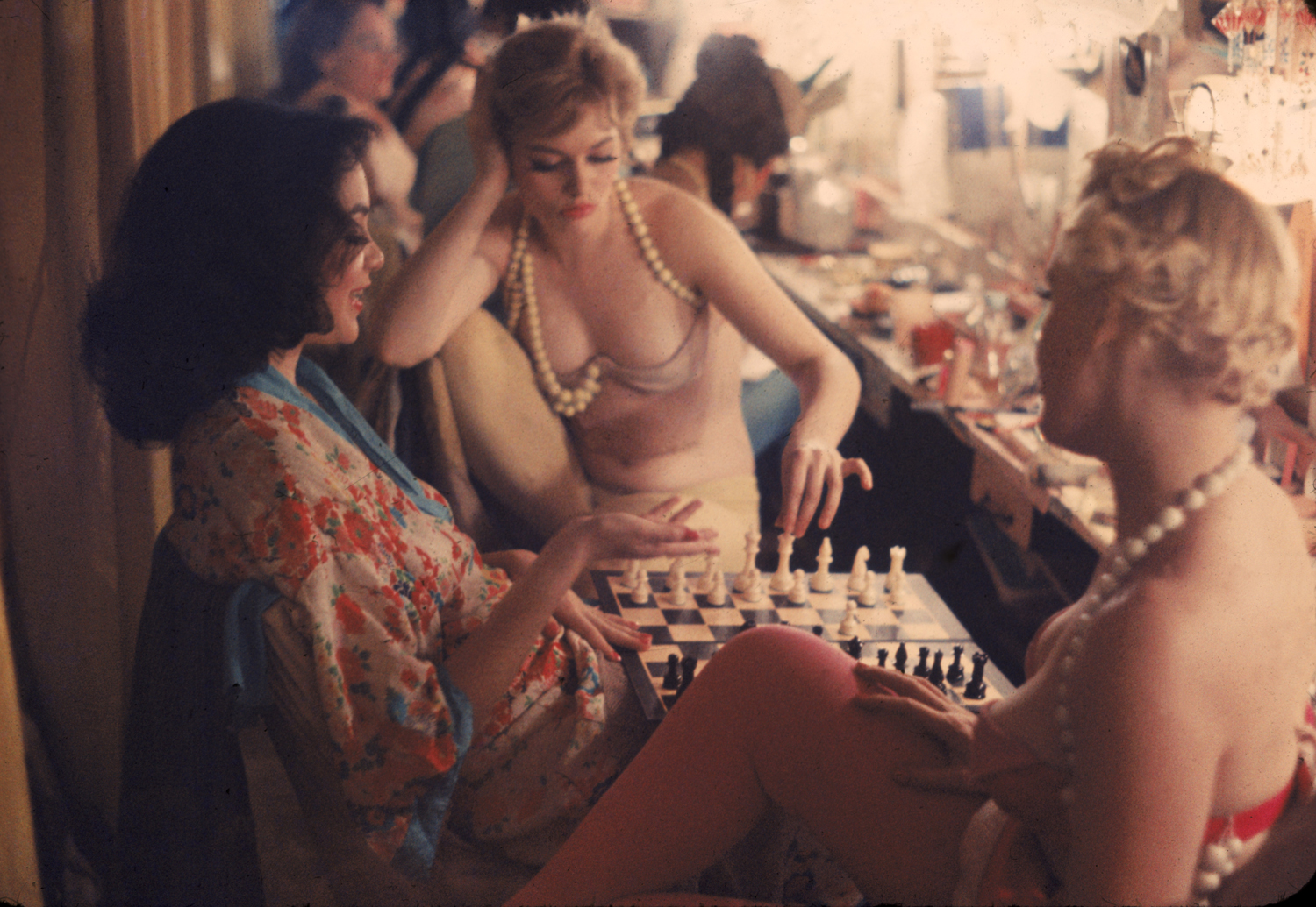
Hybrid cropping results
We’ll conclude by using the hybrid detector on several photos displaying both the features, and how this can be used to crop the photo into three different output shapes.
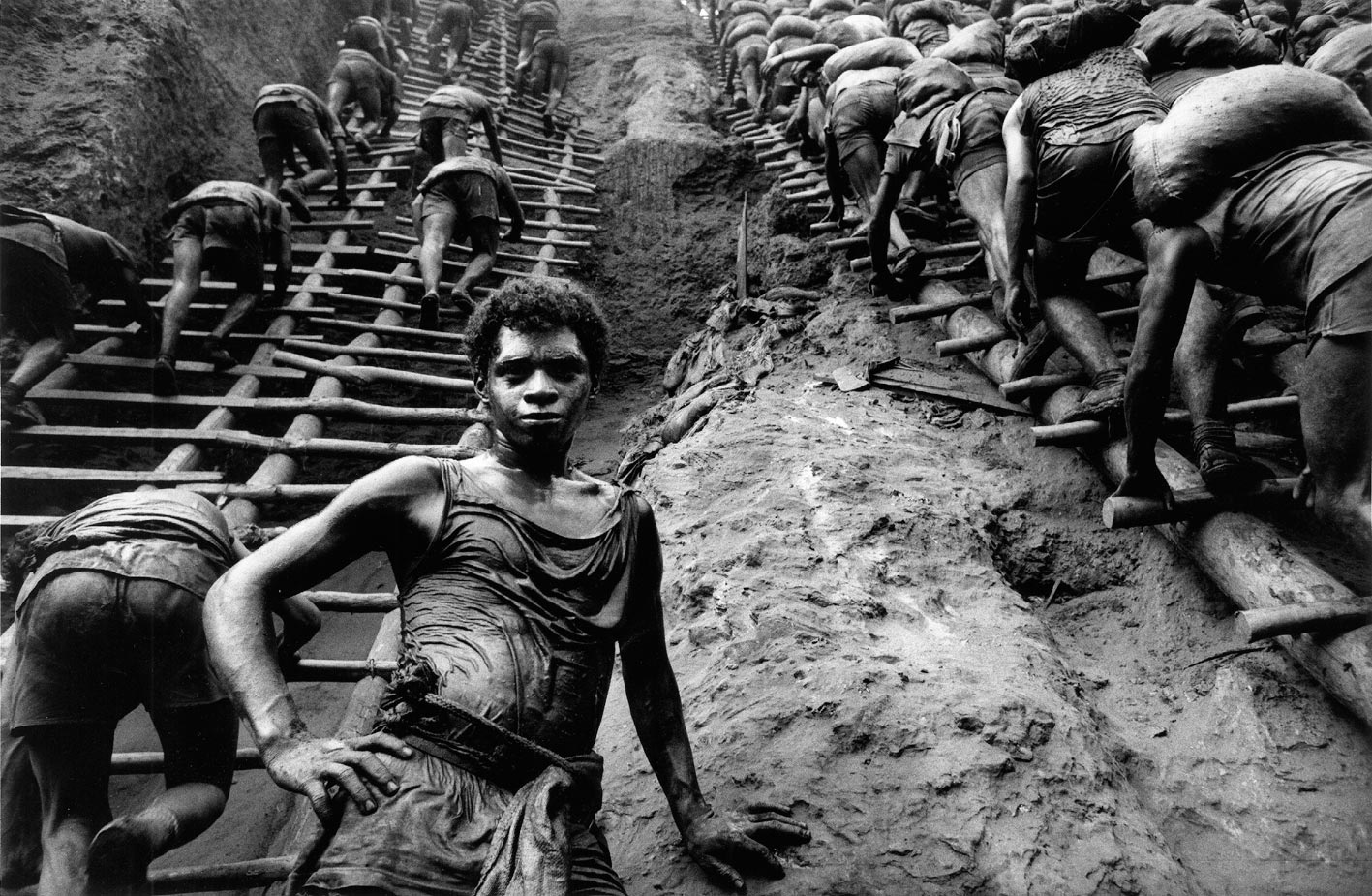
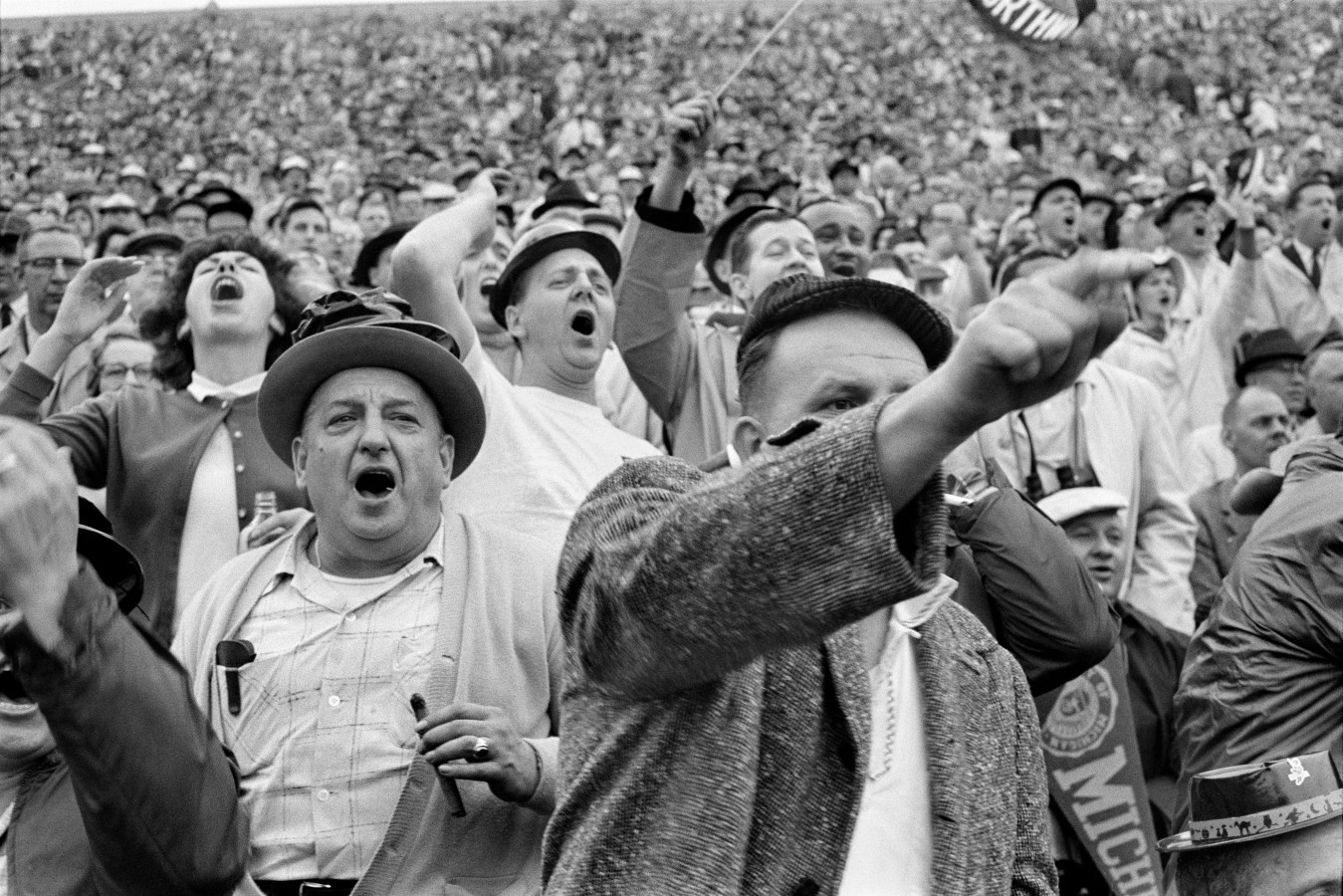
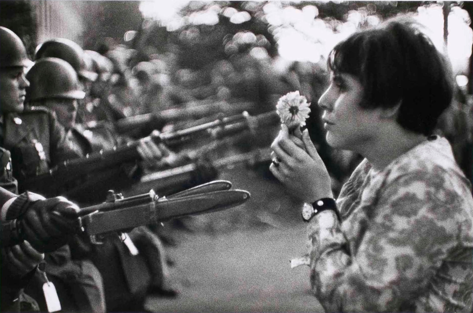
images = [
	'Sebastiao-Salgado-Serra-Pelada-1986.jpg',
	'Henri-Cartier-Bresson-Ann-Arbor-1960.jpg',
	'Henri-Cartier-Bresson-Dessau-1945.jpg',
	'monkey-race.jpg',
	'Henri-Cartier-Bresson-Hyeres-France-1932.jpg',
	'Marc-Riboud-Washington-1967.jpg',
]
detector = HybridDetector()
detect_and_show(images, detector, preview=True)